Hatching
shape-based tonal or shading

Hatching is an artistic technique that uses closely spaced or even overlapping lines to create tonal or shading effects. Here, we use the R programming language to generate a hatching-style drawing from an initial reference image.
We will first read in an image, such as the R logo image.
library(jpeg)
## sample image
img <- readJPEG(system.file("img", "Rlogo.jpg", package="jpeg"))[,,1]
img <- t(apply(img,2,rev)) ## rotate
You can plot this image to know what we’re starting with.
image(img, axes=FALSE, col=grey(seq(0, 1, length = 256)))
Note that img is a matrix, ranging from 0 to 1, with 0 being darkest and 1 being brightest. If I was making a hatching drawing by hand, I would probably first draw the lighter tones. Then I would add more and more hatches to create the appearance of darker and darker shadows. We will try to break down what we do artistically into something that can be programmatically executed by a computer.
First, I’m going to use R to draw a few random hatches sampled from the points in my image. When drawing, I naturally vary the size of my hatches. So programmatically, I’m going to randomly vary the size of the hatches using rnorm to generate these random hatch sizes.
pos <- which(img < 1, arr.ind=TRUE)

invisible(lapply(ts, function(t) {
m <- min(N, nrow(pos))
vi <- sample(1:nrow(pos), m)
pos <- pos[vi,]

## random hatch size
cex <- rnorm(nrow(pos), size, var)

## plot
plot(pos,
     pch=pch,
     col=rgb(0,0,0,0.1),
     cex=cex,
     axes=FALSE,
     xlab=NA,
     ylab=NA
)
Next, for each darker and darker shade in my reference image, I will add more hatches to that region. For example, I will take all regions in my reference image that are darker than 0.5 on our grey scale of 0 to 1 and add more hatches with the same approach described previously.
## add on shading
t <- 0.5
pos <- which(img < t, arr.ind=TRUE)

## random set of points that meet this criteria
m <- min(N, nrow(pos))
vi <- sample(1:nrow(pos), m)
pos <- pos[vi,]

## random hatch size
cex <- rnorm(nrow(pos), size, var)

## add points
points(pos,
       pch=pch,
       col=rgb(0,0,0,0.1),
       cex=cex
)
And I can repeat this for darker and darker shades.
But instead of manually picking my shading steps, I will try to sample from the distribution of shades in my reference image. So, we will need to check what grey-scale tones are presented in the reference image. I’m going to ignore the pure blacks (0) and pure whites (1).
ts <- unique(quantile(img, rev(seq(0, 1, step))))
ts[ts >= 1] <- 0.99
ts[ts <= 0] <- 0.01
Now, rather than repeating manually for different shades, I will also use a loop to keep adding more hatches for darker and darker shades.
## add on shading layers
invisible(lapply(ts, function(t) {
    pos <- which(img < t, arr.ind=TRUE)
    m <- min(N, nrow(pos))
    vi <- sample(1:nrow(pos), m)
    pos <- pos[vi,]
    cex <- rnorm(nrow(pos), size, var)
    points(pos,
           pch=pch,
           col=rgb(0,0,0,0.1),
           cex=cex
    )
}))
What this looks like all put together is:
Now, we can just read in an image and make a simple function call.
## to read in an image
library(jpeg)
## sample image
img <- readJPEG(system.file("img", "Rlogo.jpg", package="jpeg"))[,,1]
img <- t(apply(img,2,rev)) ## rotate
## call our function
hatching(img)
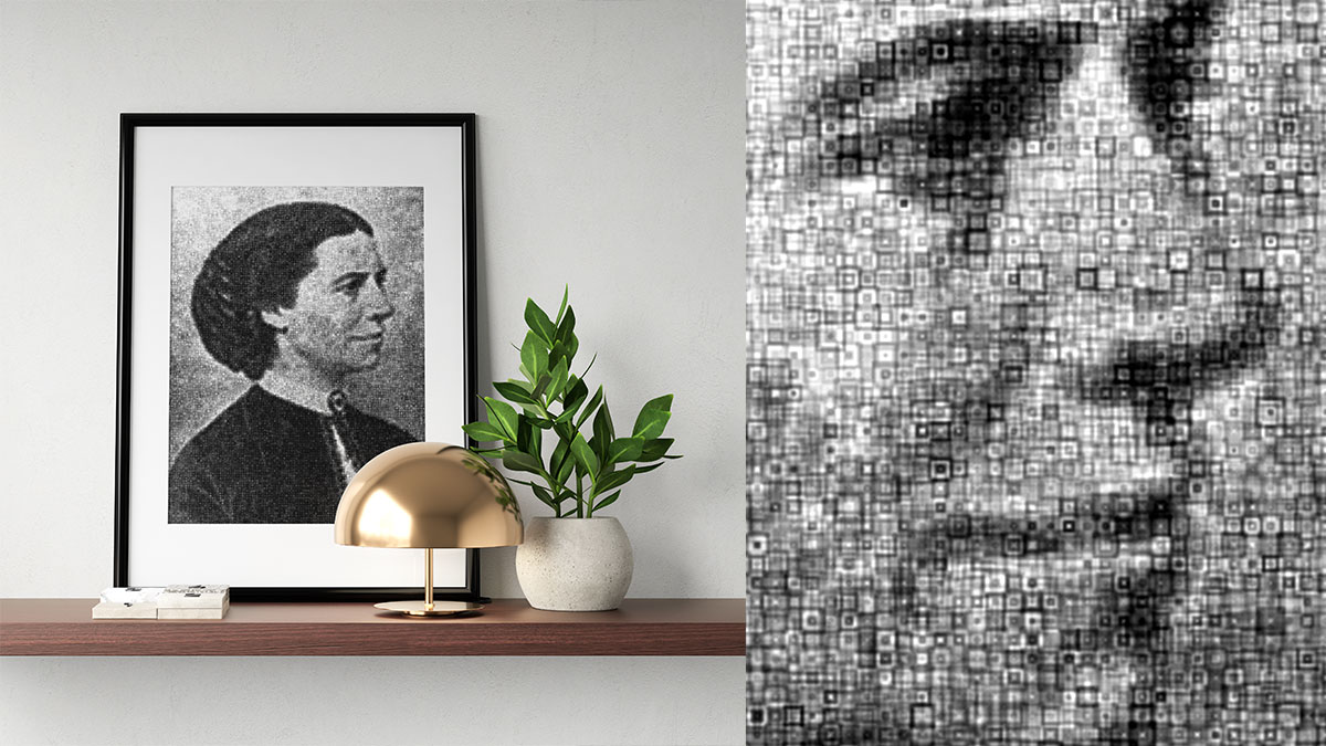
Note that we don’t have to restrict outselves to hatches. We can use any shape! Like squares!
## image of Clara Barton from Wikimedia Commons
## https://commons.wikimedia.org/wiki/File:Clara_Barton_1865.jpg
img <- readJPEG('~/Desktop/Clara_Barton.jpg')[,,1]
img <- t(apply(img,2,rev)) ## rotate
hatching(img, size=0.1, var=0.5, N=10000, pch=0, step=0.01)